Training a model for automated curation

If the pretrained models do not give satisfactory performance on your data, it is easy to train your own classifier using SpikeInterface.

Step 1: Generate and label data

First we will import our dependencies

import warnings
warnings.filterwarnings("ignore")
from pathlib import Path
import numpy as np
import pandas as pd
import matplotlib.pyplot as plt

import spikeinterface.core as si
import spikeinterface.curation as sc
import spikeinterface.widgets as sw

# Note, you can set the number of cores you use using e.g.
# si.set_global_job_kwargs(n_jobs = 8)

For this tutorial, we will use simulated data to create recording and sorting objects. We’ll create two sorting objects: sorting_1 is coupled to the real recording, so the spike times of the sorter will perfectly match the spikes in the recording. Hence this will contain good units. However, we’ve uncoupled sorting_2 to the recording and the spike times will not be matched with the spikes in the recording. Hence these units will mostly be random noise. We’ll combine the “good” and “noise” sortings into one sorting object using si.aggregate_units.

(When making your own model, you should load your own recording and do a sorting on your data.)

recording, sorting_1 = si.generate_ground_truth_recording(num_channels=4, seed=1, num_units=5)
_, sorting_2 =si.generate_ground_truth_recording(num_channels=4, seed=2, num_units=5)

both_sortings = si.aggregate_units([sorting_1, sorting_2])

To do some visualisation and postprocessing, we need to create a sorting analyzer, and compute some extensions:

analyzer = si.create_sorting_analyzer(sorting = both_sortings, recording=recording)
analyzer.compute(['noise_levels','random_spikes','waveforms','templates'])

estimate_sparsity (no parallelization):   0%|          | 0/10 [00:00<?, ?it/s]
estimate_sparsity (no parallelization): 100%|██████████| 10/10 [00:00<00:00, 535.08it/s]

noise_level (no parallelization):   0%|          | 0/20 [00:00<?, ?it/s]
noise_level (no parallelization): 100%|██████████| 20/20 [00:00<00:00, 281.93it/s]

compute_waveforms (no parallelization):   0%|          | 0/10 [00:00<?, ?it/s]
compute_waveforms (no parallelization): 100%|██████████| 10/10 [00:00<00:00, 461.81it/s]

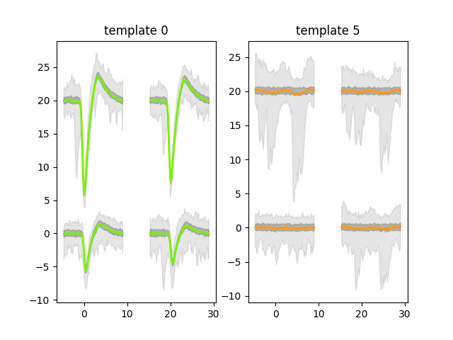
Now we can plot the templates for the first and fifth units. The first (unit id 0) belongs to sorting_1 so should look like a real unit; the sixth (unit id 5) belongs to sorting_2 so should look like noise.

sw.plot_unit_templates(analyzer, unit_ids=["0", "5"])

<spikeinterface.widgets.unit_templates.UnitTemplatesWidget object at 0x73e4c4da1ea0>

This is as expected: great! (Find out more about plotting using widgets.) We’ve set up our system so that the first five units are ‘good’ and the next five are ‘bad’. So we can make a list of labels which contain this information. For real data, you could use a manual curation tool to make your own list.

labels = ['good', 'good', 'good', 'good', 'good', 'bad', 'bad', 'bad', 'bad', 'bad']

Step 2: Train our model

We’ll now train a model, based on our labelled data. The model will be trained using properties of the units, and then be applied to units from other sortings. The properties we use are the quality metrics and template metrics. Hence we need to compute these, using some sorting_analyzer` extensions.

analyzer.compute(['spike_locations','spike_amplitudes','correlograms','principal_components','quality_metrics','template_metrics'])

Fitting PCA:   0%|          | 0/10 [00:00<?, ?it/s]
Fitting PCA: 100%|██████████| 10/10 [00:00<00:00, 176.04it/s]

Projecting waveforms:   0%|          | 0/10 [00:00<?, ?it/s]
Projecting waveforms: 100%|██████████| 10/10 [00:00<00:00, 2423.75it/s]

Compute : spike_locations + spike_amplitudes (no parallelization):   0%|          | 0/10 [00:00<?, ?it/s]
Compute : spike_locations + spike_amplitudes (no parallelization): 100%|██████████| 10/10 [00:00<00:00, 205.16it/s]

noise_level (no parallelization):   0%|          | 0/20 [00:00<?, ?it/s]
noise_level (no parallelization): 100%|██████████| 20/20 [00:00<00:00, 384.76it/s]

calculate pc_metrics:   0%|          | 0/10 [00:00<?, ?it/s]
calculate pc_metrics:  40%|████      | 4/10 [00:00<00:00, 30.20it/s]
calculate pc_metrics:  80%|████████  | 8/10 [00:00<00:00, 30.17it/s]
calculate pc_metrics: 100%|██████████| 10/10 [00:00<00:00, 30.17it/s]

Now that we have metrics and labels, we’re ready to train the model using the train_model` function. The trainer will try several classifiers, imputation strategies and scaling techniques then save the most accurate. To save time in this tutorial, we’ll only try one classifier (Random Forest), imputation strategy (median) and scaling technique (standard scaler).

We will use a list of one analyzer here, so the model is trained on a single session. In reality, we would usually train a model using multiple analyzers from an experiment, which should make the model more robust. To do this, you can simply pass a list of analyzers and a list of manually curated labels for each of these analyzers. Then the model would use all of these data as input.

trainer = sc.train_model(
    mode = "analyzers", # You can supply a labelled csv file instead of an analyzer
    labels = [labels],
    analyzers = [analyzer],
    folder = "my_folder", # Where to save the model and model_info.json file
    metric_names = None, # Specify which metrics to use for training: by default uses those already calculted
    imputation_strategies = ["median"], # Defaults to all
    scaling_techniques = ["standard_scaler"], # Defaults to all
    classifiers = None, # Default to Random Forest only. Other classifiers you can try [ "AdaBoostClassifier","GradientBoostingClassifier","LogisticRegression","MLPClassifier"]
    overwrite = True, # Whether or not to overwrite `folder` if it already exists. Default is False.
    search_kwargs = {'cv': 3} # Parameters used during the model hyperparameter search
)

best_model = trainer.best_pipeline

Running RandomForestClassifier with imputation median and scaling StandardScaler()
BayesSearchCV from scikit-optimize not available, using RandomizedSearchCV

You can pass many sklearn classifiers imputation strategies and scalers, although the documentation is quite overwhelming. You can find the classifiers we’ve tried out using the sc.get_default_classifier_search_spaces function.

The above code saves the model in model.skops, some metadata in model_info.json and the model accuracies in model_accuracies.csv in the specified folder (in this case 'my_folder').

(skops is a file format: you can think of it as a more-secure pkl file. Read more.)

The model_accuracies.csv file contains the accuracy, precision and recall of the tested models. Let’s take a look:

accuracies = pd.read_csv(Path("my_folder") / "model_accuracies.csv", index_col = 0)
accuracies.head()

	classifier name	imputation_strategy	scaling_strategy	balanced_accuracy	precision	recall	model_id	best_params
0	RandomForestClassifier	median	StandardScaler()	1.0	1.0	1.0	0	{'n_estimators': 150, 'min_samples_split': 4, ...

Our model is perfect!! This is because the task was very easy. We had 10 units; where half were pure noise and half were not.

The model also contains some more information, such as which features are “important”, as defined by sklearn (learn about feature importance of a Random Forest Classifier.) We can plot these:

# Plot feature importances
importances = best_model.named_steps['classifier'].feature_importances_
indices = np.argsort(importances)[::-1]

# The sklearn importances are not computed for inputs whose values are all `nan`.
# Hence, we need to pick out the non-`nan` columns of our metrics
features = best_model.feature_names_in_
n_features = best_model.n_features_in_

metrics = pd.concat([analyzer.get_extension('quality_metrics').get_data(), analyzer.get_extension('template_metrics').get_data()], axis=1)
non_null_metrics = ~(metrics.isnull().all()).values

features = features[non_null_metrics]
n_features = len(features)

plt.figure(figsize=(12, 7))
plt.title("Feature Importances")
plt.bar(range(n_features), importances[indices], align="center")
plt.xticks(range(n_features), features[indices], rotation=90)
plt.xlim([-1, n_features])
plt.subplots_adjust(bottom=0.3)
plt.show()

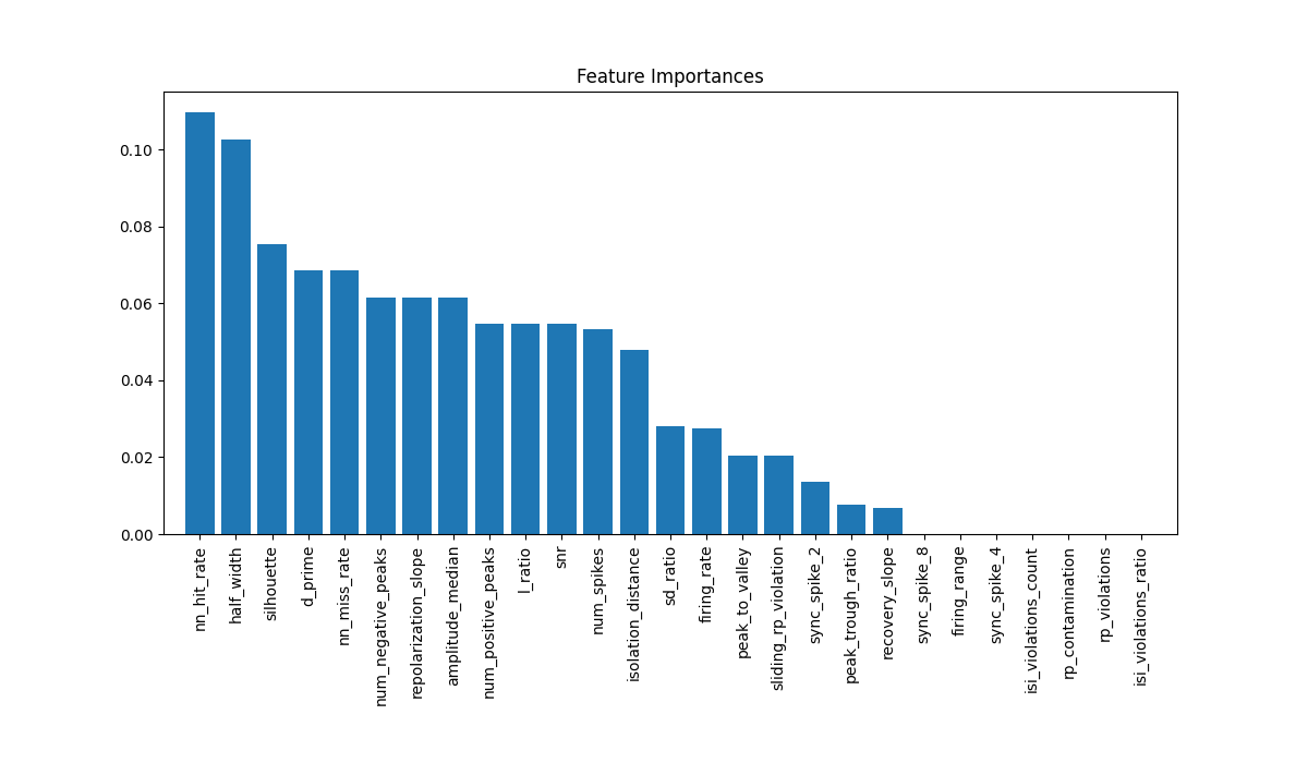
Roughly, this means the model is using metrics such as “nn_hit_rate” and “l_ratio” but is not using “sync_spike_4” and “rp_contanimation”. This is a toy model, so don’t take these results seriously. But using this information, you could retrain another, simpler model using a subset of the metrics, by passing, e.g., metric_names = ['nn_hit_rate', 'l_ratio',...] to the train_model function.

Now that you have a model, you can apply it to another sorting or upload it to HuggingFaceHub.